System evolution and biology

1. Biological systems

There are several indications that the system evolution kinetics approach applies to biological systems. According to the general definition of systems considered, such biological systems can be any living entity (bacteria, cells, organs, mammals,...) but also sub-systems in the organization of a living entity (such as the immunitary system) and super-systems as group of living entities (species, etc.). The variation of the force of mortality with time can be expressed by l(t)=dE/dt with E(t)given by Equation E-1. This corresponds to a modified Weibull distribution. Gompertz law is found back when the parameter b is made =0.

Let us just show here one example of using Equation E-1.

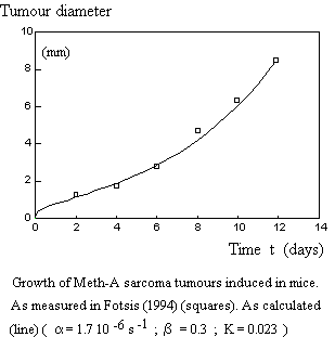
In addition, the General Adaptation Syndrome (GAS) described by Selye (1936) as a response to stress perfectly corresponds to the theory. We recall that in the GAS, one observes three successive stages: (1) adaptation ; (2) steady state ; (3) exhaustion, exactly as for the evolution of systems. Clearly, the concept "stress" used by Selye meets the constraint S due to the operation of a system in a given environment.

An article on the subject has been published in an international journal (Crevecoeur, 2001). Following article goes in the same direction : A mechanical system interpretation of the nonlinear kinetics observed in biological ageing.

2. Application to evolutionary dynamics

If biological entities can be considered as systems, then their evolution kinetics should not be contradictory to evolutionary dynamics in the Darwinian sense. Here we will give some tracks of thinking rather than to make a full demonstration.

2.1 Start of life on earth

Nei (1975) obtained a rough relationship between the number "n" of nucleotide pairs (bp) in the DNA of different species and their time of appearance on earth : n=n₀.exp (a.t), with a = 2.3 10^-9 years^-1 for an estimated 3 10⁹ years elapsed from bacteria to mammal (n₀ is the initial DNA content, e.g., 4 10⁶ bp for E. coli). This relationship is equivalent to Equation E-1 with b=0.
Assuming life to exist on earth since 3.5 10⁹ years (= zero time) and considering the appearance of (1) E. coli - 4 10⁶ bp - after 200 millions years, (2) the first unicellulars, e.g., Neurospora - 4 10⁷ bp - after 1.2 10⁹ years, (3) the bony fish - 9 10⁸ bp - after 2.6 10⁹ years and the first mammals - 3.2 10⁹ bp - after 3.1 10⁹ years, one can compare the results using Nei's equation and Equation E-1. Both equations fit the points as seen on the figure.

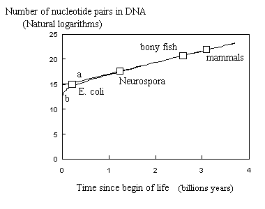
Fig. : Number of nucleotide pairs in genome as a function of time
from begin of life on earth. (a) As calculated with Nei's equation.
(b) As calculated with Equation E-1 (a=2.3 10^-9years^-1;
b= 0.45 ; K = 5.755 ). Squares correspond to 4 selected species from Nei.

However, as can be seen from the beginning of the curves (see following figure), extrapolating to point zero gives a figure of above 2 10⁶bp ( 2,525,134 bp) for Nei's equation.

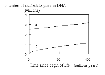Such a big number of nucleotide pairs per genome seems unrealistic directly at start of life. On the contrary, using Equation E-1 allows to start from small molecules (0 bp at time 0; 229 bp after 1 year; etc.)
Whatever the model, the curve must start from zero. With Equation E-1 and b=0.45one better understands why the increase was so quick in the beginning (see remark of de Duve) and slowed down afterwards.

2.2 Feedback loops and evolutionary dynamics

Above considerations make sense, as we can re-interpret Figure 1and Figure 2 in the scope of evolutionary dynamics. Indeed, while Figure 2 corresponds to the environmentally induced changes in living organisms, e.g., genome mutations, Figure 1 is a good scheme for the adaptation of the fittest. The struggle for life in a limited environment will advantage the individuals with the best adaptation solutions. It has been demonstrated that advantageous mutations at a given locus can happen in specific stress conditions (environmental changes) much more often than in neutral conditions (Cairns et al., 1988 ; Hall, 1990). The positive feedback loops corresponding to an increased number of events (defects, mutations, etc.) in reaction to the environmental challenges induce adaptative efforts within the system (negative feedback loops), which can lead at a critical level to the emergence of a new behaviour or entity. This enlightens why ageing curves are applicable to evolutionary dynamics.

2.3 Step-by-step evolution

However, strongly advantageous solutions take time to become generalized to a whole population. So, the process will not occur in a continuous manner, but rather step by step. This is visualized in next figure.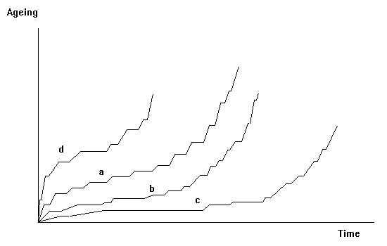

Curve "a" will correspond to a regular evolution, curves "b" and "c" to slow evolutions in the beginning with some long periods without apparent evolution, while curve "d" would be typical for a rapid evolution in the beginning (e.g., due to severe challenges), which will end in a shorter duration of the whole process. Probably what is known as the "cambrian big bang" or the "cambrian explosion" of number of species is a step of exceptionally high amplitude which occurred in the development of life. Steplike evolution curves are what one encounters in nature when the attention is focussed on particular time intervals. Equation E-1 is the envelope over all time intervals of a given process. Steplike life curves are in perfect agreement with Eldredge and Gould's theory of "punctuated equilibrium" (1972). It is interesting to draw a parallel with the experimental work of Lenski and coworkers (Lenski and Travisano, 1994 ; Elena et al., 1996). These teams followed evolutionary changes in bacterial populations (E. coli) propagated for 10,000 generations in identical environments. They first showed that cell volume and relative fitness (to the ancestor) grew according to a concave (from below) curve (Lenski and Travisano, 1994). Such curves are similar to the first part of Figure 3. But, focussing on a population at a smaller time scale (3,000 generations), they got a better fit with a step model, what they considered to show evidence of punctuated equilibrium (Elena et al., 1996). This confirms our interpretation of the ageing curve as the large scale envelope of evolutionary dynamics through punctuated equilibrium (compare Figure 3 to Figure 3.1 and Figure 3.2). It is thus a way to reconcile the followers of Gould and Eldredge with those who see evolution as a continuous process: the difference is in the time scale considered. Thus the adequacy of the chosen time scale is a key element for correct interpretation in evolution dynamics as it is in investigations on ageing.

Back to Home page