System evolution and the theorem of minimum entropy production

1. Concept of Self-Organized Criticality

Self-organized criticality (or "SOC") is a concept invented by Bak and co-workers (1987) on base of observations on sandpiles and computer simulation of cellular automata. According to this concept, many composite systems naturally evolve towards a "critical" state characterized by four facts:

minor events can be at the origin of chain reaction which can affect any number of elements in the system: therefore, "avalanches" of events of any size can be produced ;

the sizes of the avalanches are statistically distributed according to a power law with a negative exponent of the order of ...1...2...

this is true as well in space as in time ;

when the system is constrained to produce events, it tends, thanks to the avalanches, to return to a steady state of criticality (therefore, the expression "self-organized criticality").

In the system evolution kinetics approach, all systems are by definition in a state of SOC.

The statistical distribution of avalanches of events according to a power law is used to characterize "b_(i)" in the equation for the negative feedback loops (adaptations).

2. Phase space

In statistical mechanics, a system can be represented by a volume "V" in the phase space. This volume includes the probability of position and quantity of motion of all points of the system at a given time. Its time evolution will be given by the time evolution "V(t)" of its representative volume. Starting from a given volume at time zero, the time evolution of the system is represented by the beam formed by all possible trajectories followed by its unitary components with time. This beam will be restricted to a part of the phase space because: (1) the system is a whole of interlinked subparts (some trajectories are prohibited because the system operated as a whole) and (2) there might be external constraints (limiting the liberty of movement of the system).

3. Boltzmann's entropy

The relevant entropy for understanding the time evolution of systems is Boltzmann's entropy "S_B" (see Lebowitz,1993). Boltzmann's entropy defines the relationship between "S_B" and "V" at a given time by:

This equation holds in time:

Indeed, after a small increment of time "dt", Boltzmann's entropy will have changed by "dS_B" and the volume in the phase space by "dV". We have (using a Taylor development in series):

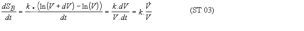
and, after integration supposing the functions "S_B(t)" and "V(t)" to be continuous, we obtain equation ST02 save on a constant term. We then get a beam of possible trajectories.

4. Theorem of minimum entropy production

The theorem of minimum entropy production of Prigogine (1961) states that the variation of the entropy production over time is negative or zero in non-equilibrium stationary states not far from the equilibrium.

5. Statistical ageing or evolution

Let us apply the theorem of minimum entropy production to Boltzmann's entropy as it is this entropy which applies for evolving systems. The simplest way to analytically express the theorem and have the entropy always positive or zero is given by following equation:

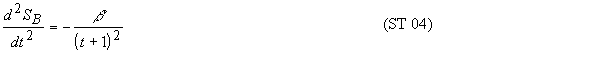
with "b'" constant.

The variation of entropy production will then be minimum at complete equilibrium, ie. at "t" infinite. One writes "t+1" instead of just "t" to avoid getting a logarithm infinite negative after double integration. If the time is expressed in units of Planck's time, adding "1" just means that we start to analyze the system's evolution one unit of Planck's time, ie. as soon as 10^-43seconds after start. This makes sense as this is the time limit given by quantum mechanics for physical observations (see also Nottale).

When integrated one time, equation ST 04 gives:

with "a'" the integration constant.

When integrated, equation ST05 gives:

with "k'" the integration constant.

Therefore, "V(t)" is given by:

with: K=k'/k, a=a'/k and b=b'/k.

This is Equation E-1 as the value "1" can be neglected in most applications, being Planck's time, ie. something extremely small compared to present measurement accuracies.

In equation ST 04, zero is obtained in two particular cases: t = infinite (the evolution is purely adaptive if "a" is nil ; it is more complicated and goes towards an end if "a" is different from zero) or "b"=0 (the evolution is exponential if "a" is different from zero, it is nil when "a" is nil).
For the class of systems under scope, observation shows that b lies between 0 and 1, ie. b' is less than k.

Back to Home page